Home » Examples » Shock Response for Equipment Response to Impulsive Loads

Shock Response for Equipment Response to Impulsive Loads

Shock response is important for understanding equipment’s response to impulsive loads. An impulsive load can be anything from a mechanical impulse to a water hammer, travelling across road bumps or drops, shock pulses, and explosions. Equipment response includes a variety of systems, e.g. electric cabinets, satellites, motors, generators, coolers, piping, cardboard boxes containing goods, and sensor response.

Shock response results can be confusing, as they show response versus resonance frequency. We need to elaborate a bit on the basics behind shock response to be able to discuss and explain it fully. Correctly measuring shock requires an understanding of sensor characteristics, as well as an understanding of some of the basics regarding the transient excitation of resonant systems.

To be able to follow this text, the reader should understand the SDOF system (see basics for the sdof). Furthermore, the reader should understand the basics of Fourier Transform, signal analysis, and filters (see the Signal Analysis subsection). It would also be helpful to understand how vibration sensors function (see the Sensor section).

Note that the subject of shock response is vast, and that this text will focus only on the basics. See the end of this post for links for more advanced reading on the subject.

The simplest mechanical impulse is the half sine wave, as shown in Figure 1. The rule of thumb is that a short duration event of duration dτ and amplitude A shows a fixed amplitude A up to the frequency ~1/dτ, and that 90% of the impulse energy is found at frequencies below ~2/dτ, as shown in Figure 1.

Figure 1. Half sine wave and corresponding spectrum (Click on Figure to enlarge)

The simplest dynamic system is the SDOF system. A SDOF systems can be used to represent most linear systems using so-called Modal base functions. The SDOF system is comprised of three elements— a mass, a spring that connects to the base, and a damper. The SDOF system can be excited either by the direct application of force to the mass element or by vibratory base motion.

Figure 2. The Single Degree Of Freedom (SDOF) system has three elements, a mass, a spring and a damper. (Click on Figure to enlarge)

The observant reader may already have noticed that the half sine wave pulse very much resembles the pulse caused by a speed bump. Furthermore, the mass spring system is a very crude model of a car, truck, or bus where the mass is the vehicle’s body, the spring is the combined stiffness from suspension, and wheels and the dampers are the shock absorber.

Most people know that when driving a vehicle slowly over a speed bump, it will travel over the bump much like when travelling over a hill, i.e. with minimal compression of the the suspension spring and maximum amplitude variation for the person who rides over the bump.
Conversely, when driving across the speed bump at high speed, the vehicle suspension will absorb the bump’s motion and the vehicle body and driver will more or less remain at the height they were when the bump was approached.
It is perhaps less well known that there is a speed at which the car will show maximum bounce when passing over the speed bump. This condition occurs when the time of driving over the bump matches half the period time of the vehicle suspension’s natural frequency.

It may be hard to believe, but this behavior of a car from speed bump base excitation outlines the basic response for any dynamic system that is exposed to shock loads.

As outlined in the SDOF system theory:

There is a natural frequency f₀ for a SDOF system. At this frequency, a response is damping controlled and is said to be resonant.
At frequencies lower than ~f₀/3, the system is quasi-static, i.e. it behaves as if there is no movement.
At frequencies higher than ~f₀/3, the system is mass controlled, i.e. it is the mass that decides the response.

To continue, frequency is low and high when compared with the SDOF system’s natural frequency at quasi-static and mass controlled conditions, respectively.

The above implies that at quasi-static conditions (low frequency) when a load is applied to the mass, it is transmitted to the base to the spring and, consequently, the mass does not move much. Similarly, for quasi-static conditions, when the base moves, the mass moves nearly as much as the base and, consequently, the spring compression (load) is small.

At high frequency, the mass accommodates almost all the load that is directly applied to it and its response can be approximated using Newton’s 2nd law (Force = Mass·Acceleration). Consequently, the spring element transmits little force—the system is vibration isolated, as it does not transmit the load. For high frequency base excitation, the mass element remains more or less stationary, so the spring must accommodate the base motion amplitude. Consequently, the spring shows its maximum compression and, therefore, a load would be approximated by calculating the spring stiffness mulitiplied by the base displacement amplitude.

For stationary vibration, the SDOF system shows it highest response when it is excited at a frequency f = f₀, which (of course) implies that the period of excitement for time T matches the SDOF system’s natural period for time T₀. For shock response analysis, the maximum SDOF system response is found when the impulse duration dτ matches T₀/2 as closely as possible. This insight applies for any single impulse shape, i.e. for rectangular, triangular, half sine or versed sine pulses. As this situation is as close as possible to being resonant, the response will be affected by the SDOF system damping.

Next, the impulse duration, dτ, can be long or short when compared with T₀/2.

A long duration load would place a static force onto the mass element. Such a load would be a step type load and the response be quasi-static, i.e. a low frequency response.
A short duration load would be a so-called Dirac pulse, i.e. an infinitely short pulse, or any pulse that loads the SDOF system for a much shorter time than T₀/2. The SDOF system response would be mass controlled, i.e. a high frequency response.

As mentioned above, the SDOF system can be excited either by the direct application of force to the mass element or by vibratory base motion. Important components in the analysis include the relative base-mass motion, the spring/damper load force, the absolute motion of the mass element, or the mass force. Surprisingly, most of these combinations can be understood using two simple transfer functions, as shown in Figure 3.

(A)

(B)

Figure 3. A) Transmissibility from direct excitation, i.e. the curve demonstrates transmissibility from direct force excitation to the mass element, as well as vibration transmissibility in the case of base excitation. B) Response Transmissibility. This transfer function demonstrates the response of the mass element from direct force excitation to the mass element, as well as the relative motion between mass element and base in the case of base excitation. (Click on Figure to enlarge)

Combining the spectrum of a pulse with the above Transmissibility curves allows us to recast our earlier exploration of the car travelling across the speed bump into a general formulation.

A long duration/low frequency impulse transmits all force across the spring element and implies a small mass-base relative displacement, and a small load, as spring compression is small. It is the load magnitude and the system spring that govern the system response. l
A short duration/high frequency impulse takes up all force at the mass element and implies that the spring must accommodate the base motion amplitude. It is the load and the system mass that govern the system response.
A pulse half period that is adapted to the system’s natural frequency produces maximum system response, and this response is affected by the system damping. It is the load and the system damping that govern the system response, which is maximum for a given load amplitude.

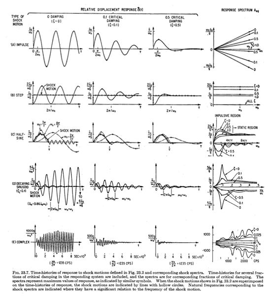
The above is the spectral interpretation, but, as excitation is transient, the response should be analysed in the time domain. Figure 4 shows system response from generic impulse shapes.

(A)(B)

(C)

Figure 4. A) SDOF system response from generic types of transient excitation. Figure from Harris’ shock & vibration handbook. (Click on Figure to enlarge). B) Time response due to various impulsive (short duration) loads. We see that response is similar for all cases in the impulsive region. C) B) Time response due to various static (long duration) loads. We see that response is similar for all cases in the static region.

At this time, we will use the above insights to discuss sensor response and sensor selection.

An accelerometer uses a small sensor mass placed on top of a piezoelectric crystal or a strain gauge bridge to generate a signal proportional to its base acceleration.
- The accelerometer therefore has as high a natural frequency as possible in order to give it as wide a true frequency range as possible.
- A short duration shock excites from 0 Hz to high frequency. Therefore, the accelerometer response is severely degraded if flexibility is introduced between the sensor and the measurement object, as this lowers its mounted resonance frequency.
A seismometer and a vibration velocity sensor works in the opposite manner, as the sensor has a coil placed in a magnetic gap (like a loudspeaker element) and uses the relative base-mass motion to generate a signal proportional to the base vibration velocity.
- The seismometer and a vibration velocity sensor therefore only measures vibration velocity correctly at high frequencies, i.e. at frequencies well above the sensor resonance frequency.
- This works fine for stationary signals such as machine rotation, but is inconvenient for transient vibration, as a shock invariably drives the sensor in its low frequency region, where its response is underestimated, as well as driving the sensor at its half period, where response is overestimated and depends on the sensor’s built-in damping.
- To overcome this problem, the sensor transfer function has to be measured and special filters tuned to the sensor response can be used to compensate for the sensor error (this procedure is called also inverse filtering).
- Incorrectly tuned filters add error to the operation, and compensation can never be made for cross axis sensitivity which may affect end results.
- As no sensor has exactly the same resonance frequency and damping, the tuned filter must be tuned for each sensor, and compensation typically is made after the measurement. This topic is discussed at length here (**).

The above highlights and explains why the accelerometer truly is the sensor of choice whenever transient measurement is concerned, and why the accelerometer must be firmly attached to the test object.

In fact, for very strong shocks, strain gauge based accelerometers tend to be favored over piezoelectric ones, as a strong shock pulse can rearrange the crystal molecule structure, leading to sensor errors that affect the result when response is integrated from acceleration to velocity or displacement. The sensitivity to this molecule structure varies with accelerometer type. Therefore, dedicated shock sensors, i.e. sensors truly designed for strong shock measurement, should be used in shock test machines, while general acceleration sensors may be used for a vibration table and for moderate shock strength on ordinary equipment.

To continue, the above outlines the basic physics of shock excitation and system response. The reader should by now be aware that there is a case where any pulse of finite duration produces a maximum system response, namely that where the effective pulse length matches the resonant system’s half period. This insight forms the basis of the so-called Shock Response Spectrum (SRS) and the Response Spectrum (RS) where the frequency axis is (confusingly) called resonance frequency and several curves are shown for various loss factor (or Q-factor) values, as shown in Figure 5.

The resonance frequency and Q-factor refer to that of the SDOF system the time signal is convoluted with and the SRS/RS amplitude refers to the maximum amplitude of the SDOF response. Note that a single SRS value is the result of a long time series being convoluted with a specific SDOF resonance frequency and Q-factor combination, i.e. the SRS is a very strong data reduction technique as can be seen in Figure 5(C).

To continue, we must first make the distinction that the RS refers to relative mass-base motion and force transmission, whereas SRS refers to absolute motion, i.e. the response of the mass element and the load accommodated by the spring element. Next, we must remember that the maximum response is when the effective pulse length matches that of the system resonance’s half period.

Now, for a complex transient load sequence—say, an earthquake, or the combination of the 1000 worst load cases of a package being transported—it is not directly obvious which portion of this signal excites the system the most strongly, nor is it realistic to assume that the system has only a a single resonance (a single mode of vibration). We can therefore combine the transient load sequence with the response of a SDOF system to estimate the maximum response. It is this procedure that produces the SRS and the RS, and these fields specify the maximum modal response.

To summarize. So far, we have discussed how to derive the SRS/RS from a set of one or more transient signals. Below, we will discuss how to use the RS/SRS once it has been derived.

(A)

(B)

(C)

Figure 5. Example of shock response spectrum (A) Transient signal is convoluted by SDOF system with the loss factor 1/Q maximum impulse response to produce the shock response spectrum (SRS). Note that the time signal must be convoluted per SDOF resonance frequency to build up the SRS spectrum for a single loss factor 1/Q. (B) SRS with different SDOF Q-values. (C). SRS for 584 hrs of time data of XYZ direction response. (Click on Figure to enlarge)

SRS as shown in Figure 5 can seem confusing at first, but produce a very convenient way of estimating maximum system response of a new, not yet existing structure. They also allow for the combination of multiple excitation types into a single equivalent spectrum.

Next, imagine that we have a set of system modes, e.g. from Experimental Modal Analysis or from Finite Element analysis. The response of these modes can thereafter simply be scaled by the SRS and RS spectrum response to produce estimates for maximum vibration, maximum stress, interface load, and so on. This is a great simplifying step, as detailed analysis of the system response would be time consuming, and would also fail to produce conservative response/load estimates.

However, when there are multiple modes in the system, their responses will interact and combine. For closely located modes, the response can be estimated using the assumption that their energies combine, i.e. by combining their RMS values as 〖RMS〗_ab^ =√(〖RMS〗_a^2+〖RMS〗_b^2 ). This assumes the responses to be uncorrelated, which they are when viewed over a period much longer than the longest system period time, but it ignores the fact that peak amplitudes may overlap. This procedure, therefore, underestimates the system peak response.

Another way to exploit the insights explained above is when making component testing on a vibration table. In this situation, we have a SRS/RS defined for the test, and we simply input this spectrum as a random signal to the system for a long enough time to establish a stationary response and a relevant number of load cycles. The system response is then measured, and the component can be examined for malfunction during the test, e.g. if it is an electronic PLM controller.

For low load cases, e.g. package drop or pyrotechnic shocks, the procedure is to first vibrate the component and experimentally identify its dominant natural frequency. The drop test pulse thereafter is tuned as closely as possible to match the system’s half period. Tuning is typically done by placing elastic inserts between the component and the shock test machine.

Finally, a long time sequence that is rain flow filtered can be converted into a new damage equivalent time signal, which in turn is analyzed and turned into a damage equivalent SRS/RS.

As mentioned above, this post covers only the broad topics and basic insights for this field to serve as an overview and appetizer for the curious mind. The curious reader can find more in-depth descriptions on shock response analysis here (shock response tutorial) and here (B&K Mechanical Vibration and Shock Measurements). In addition, newer versions of the basic reasoning behind shock response analysis have been developed over time. Several more modern versions can be found here (Dynamic Environmental Criteria: NASA Technical Handbook).